
Have you ever wondered how a car’s speedometer relates to the distance it travels? Or how the journey of a rocket launching into space can be represented on a simple chart? The answer lies in the powerful relationship between distance, time, velocity, and the graphs that depict these concepts. This article will dive into the fascinating world of distance-time and velocity-time graphs, exploring their fundamental principles, practical applications, and how they unlock a deeper understanding of motion.

Image: www.vrogue.co
Understanding these graphs is not simply an academic exercise; it is a key to comprehending the world around us. Imagine you’re watching a race. The commentator might say, “The runner is gaining speed!” But how do they know? They’re observing the runner’s velocity, which is determined by the relationship between distance and time. By analyzing the graphs, we can glean crucial insights into the motion of objects, from simple everyday examples to complex scientific phenomena.
The Foundation: Distance and Time
To understand the graphs, we must first define our terms:
-
Distance: The total length traveled by an object. Imagine a car driving from point A to point B. The distance is the direct path traveled, regardless of any detours.
-
Time: The duration of the motion. It’s the time elapsed from the start of the journey to the end.
Distance-Time Graphs: These graphs are visual representations of an object’s movement over a specific period.
- Horizontal Axis: Represents time (t)
- Vertical Axis: Represents distance (d)
Understanding Distance-Time Graphs
Let’s illustrate this with an example: A car travels at a constant speed of 50 km/h for two hours. Here’s how we would represent this journey on a distance-time graph:
-
Plotting the Points: At time 0 (the start), the car is at a distance of 0. This is our first point (0, 0). After one hour, the car has traveled 50 km (50km/h x 1h = 50km). We plot this as (1, 50). After two hours, it’s at 100 km (50 km/h x 2h = 100km) giving us (2, 100).
-
Connecting the Dots: Connect the plotted points with a straight line. This line represents the car’s journey.
Interpreting the Slope: The slope of the line on a distance-time graph tells us the object’s velocity. A steeper slope indicates a faster velocity. A horizontal line means no movement. A downward slope indicates a return journey.
Velocity and its Time-Based Representation
- Velocity: The rate of change of distance over time. It measures how fast an object is moving in a given direction. Unlike speed, which only considers magnitude, velocity takes direction into account. For example, 20 m/s north is different from 20 m/s south.
Velocity-Time Graphs: These graphs depict how an object’s velocity changes over time.
- Horizontal Axis: Time (t)
- Vertical Axis: Velocity (v)
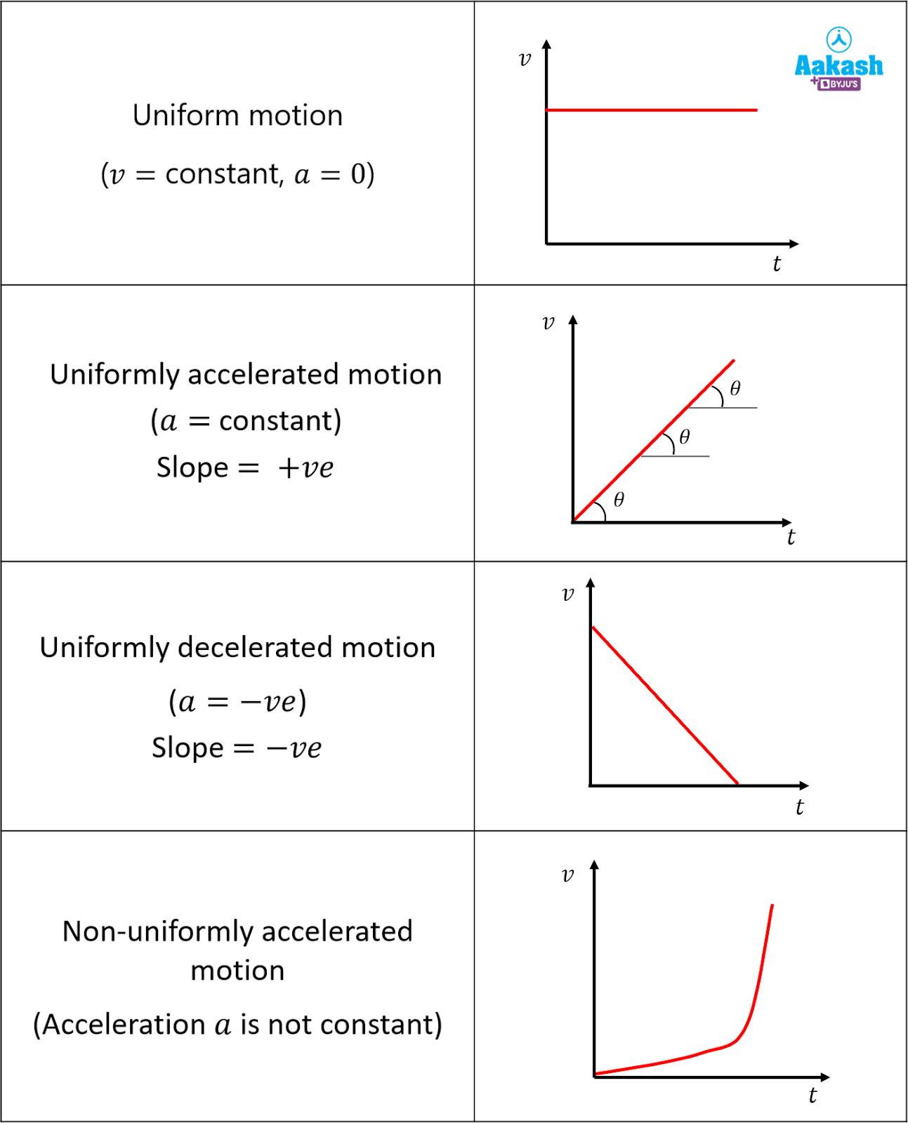
Image: www.animalia-life.club
Understanding Velocity-Time Graphs
Let’s consider the same car example as before, but this time we’ll focus on its velocity:
-
Plotting the Points: The car travels at a constant speed of 50 km/h throughout its journey. This means its velocity remains constant. We can plot this as a horizontal line at 50 km/h on the graph. No matter how much time passes, the velocity remains constant.
-
Interpreting the Graph: From the velocity-time graph, we see that the car’s velocity is unchanging. The slope (or lack thereof) of the line represents the acceleration of the object. A constant velocity implies zero acceleration.
The Link Between the Graphs
Distance and velocity graphs are inherently connected. The area under the velocity-time graph represents the total displacement of the object.
- Example: If we calculate the area of the rectangle under the constant velocity line (50 km/h x 2 hours = 100 km), we get the total displacement, which is the same as the total distance covered in our previous distance-time graph.
Going Beyond the Basics: Applications in the Real World
The concepts we’ve learned have profound real-world applications:
-
Sports Analysis: Using distance-time and velocity-time graphs, coaches can analyze athletes’ performance and identify areas for improvement. For example, they can determine a runner’s top speed and acceleration, or a swimmer’s pace throughout a race.
-
Traffic Engineering: By studying traffic flow using these graphs, engineers can design more efficient road networks, optimize traffic light timings, and implement speed limits to reduce congestion and accidents.
-
Space Exploration: These graphs are crucial for tracking spacecraft during launch and flight. Analyzing a rocket’s velocity graph can reveal if it’s reaching the necessary speed for orbit or facing issues like engine failure.
-
Weather Forecasting: Meteorologists use these graphs to track the movement of storms and predict their path and intensity.
Key Takeaways
Distance-time and velocity-time graphs provide a powerful visual language for understanding motion and its characteristics, enabling us to:
-
Analyze Motion: By interpreting the slope and area of these graphs, we can glean insights into speed, acceleration, displacement, and other aspects of motion.
-
Improve Performance: These graphs help optimize performance in fields like sports, transportation, and scientific research.
-
Make Data-Driven Decisions: They offer valuable information for decision-making in diverse applications, ranging from everyday transportation to complex space missions.
Gizmo Distance Time And Velocity Time Graphs Answers
Exploring Further
The world of graphs extends far beyond these two basic types, but understanding them is a critical starting point. For those interested in delving deeper, consider exploring topics like:
- Acceleration-Time Graphs: These graphs reveal how an object’s acceleration changes over time. They are crucial for understanding forces acting on an object.
- Graphs in Three Dimensions: Real-world movement often involves more than just one dimension. Three-dimensional graphs can visualize motion in more complex scenarios.
- Using Technology for Graph Analysis: Software tools and apps can simplify the creation and analysis of motion graphs, making them accessible for everyday use.
We encourage you to investigate these rich areas of study and see how these fundamental tools can illuminate your understanding of the world around you.


